Description

Introduction

This task will use some technique to understand the dataset, then will used machine learning technique for predict outlet sales based on the Big Mart Sales Dataset. There are many machine learning techniques that used for prediction like Decision Trees, Linear Regression, Neural Network, Support Vector Regression, etc. This task will focus on sales prediction using some of the machine learning techniques above. But before doing prediction using machine learning, we will do some visualization and some technique to understand the dataset and to know the correlation between independent variable and dependent variable.

Data Description

The data scientists at Big Mart have collected 2013 sales data for 1559 products across 10 stores in different cities. Also, certain attributes of each product and store have been defined. The aim is to build a predictive model and predict the sales of each product at a particular outlet. Using this model, Big Mart will try to understand the properties of products and outlets which play a key role in increasing sales. Sales of a given product at a retail store can depend both on store attributes as well as product attributes. The dataset is ideal to explore and build a data science model to predict the future sales. The dataset provides the product details and the outlet information of the products purchased with their sales value in the CSV file format. This dataset have 11 independent variables and 1 dependent variable. The variable description can be seen below:

• ProductID: unique product ID
• Weight: weight of products
• FatContent: specifies whether the product is low on fat or not
• Visibility: percentage of total display area of all products in a store allocated to the particular product
• ProductType: the category to which the product belongs
• MRP: Maximum Retail Price (listed price) of the products
• OutletID: unique store ID
• EstablishmentYear: year of establishment of the outlets
• OutletSize: the size of the store in terms of ground area covered
• LocationType: the type of city in which the store is located
• OutletType: specifies whether the outlet is just a grocery store or some sort of supermarket
• OutletSales: (target variable) sales of the product in the particular store

Data Understanding

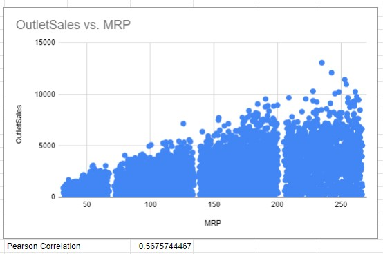
In the beginning, data understanding is needed to know the dataset and to know what can we do using the dataset. So in this part, some observation was done like visualization data to make the hypothesis of the correlation between independent variable and dependent variable (using scatter plot). Not only visualization, we also using Pearson Correlation to make sure the correlation between independent variable and dependent variable where the Pearson Correlation score near 0 means the variable has week correlation with dependent variable, the Pearson Correlation score near 1 means the variable has strong positive correlation with dependent variable and the Pearson Correlation score near -1 means the variable has strong negative correlation with dependent variable.

            The figures above show visualization using scatter plot and Pearson correlation score between some independent variable and dependent variable. Based on the results only MRP has score above 0.5 that means MRP has correlation with outlet sales.

Preprocessing

After understand the data, we do some preprocessing technique to prepare the dataset. First step, remove missing value in the dataset. Second step, describe the dataset. Third, delete some columns that feel uncorrelated like product ID, Outlet ID, and Establishment Year. Forth, Label Encoding refers to converting the labels into a numeric form so as to convert them into the machine-readable form. In this dataset we convert some variable like Fat Content, Product Type, Outlet Size, Location Type and Outlet Type.

Figure 1. Remove Missing Values

Figure 2. Describe Dataset

Figure 3. Delete Some Columns

Figure 4. Label Encoding

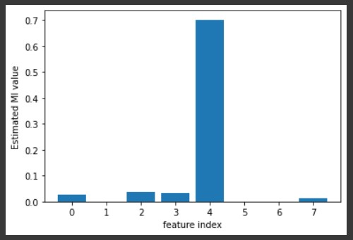
Then, Feature Selection using two methods, Feature selection using the Correlation matrix and Feature selection using the Mutual Information metric. Last, Normalized the data and split train data and test data that will used to make predicting model.

(a)

(b)

Figure 5. Feature Selection. (a) Correlation matrix (b) Mutual Information

Figure 6. Normalized Data using Min-Max Normalization