Description

THIS PORTFOLIO IS FOR DSBIZ CERTIFICATE EXAMINATION

STEPS TAKEN FOR PREDICTING USA HOUSING PRICE

DATA UNDERSTANDING
First, we need to get better understanding about the dataset that we are going to use for our data science case. We are going to use Jupyter Notebook from Google Colab to code.

1. Connect to Google Drive
   
2. The download result of USA Real Estate dataset will come out in zip file, so we need to extract it using the code below.
   
3. Read the dataset from our google drive using pandas library. This library is used for manipulating and analyzing data. Then, we're going to view the data to get the holistic view of the attributes and the values contained in every attributes. In this situation, we can see the dataset into the form of data frame to be used in Data Preprocessing or other stages in Data Science.
   
4. View the first five rows of data frame using .head() function.
   
5. Get the dimensionality of dataset using .shape, and it turns out that this dataset have 306000 columns and 10 rows.
   
6. Get the detail information of dataset, such as the number of entries or rows data, column names together with the quantity of non-null values and type of data using .info() function.
   
7. View the central tendency of dataset, such as count, mean, minimum, maximum, standard deviation, and 25%, 50%, 75% percentile using .describe() function.
   

UNIVARIATE ANALYSIS

We will do univariate analysis for every variables/attributes using histogram. This histogram will show us the frequency of data represented with rectangle bars. To plot the histogram, we need to call the matplotlib, seaborn, and plotly libaray. These libraries are used for visualize the data. For the plotting, I use two different approaches. Here is the histogram created:

DATA PREPARATION

Because real-word datasets often contain missing value due to various reason such ass data entry error, incomplete data collection, etc; we need to do preprocessing the data to transform raw data into a clean, structured, and usable format before feeding it into machine learning algorithms.

1. First, we need to check if there are missing values and outliers in our dataset. We can use .isna().sum() function to check the availability of missing values. It turns out that we have 7 attributes that contain missing values.
   
2. There are two ways to handle these missing value: drop rows/data that have cells with missing values, or fill the missing values with values obtained using descriptive statistics or Machine Learning Approach. We will use .dropna() function to drop any rows with missing values. Also, we will remove prev_sold_date attribute from dataframe because it contains a substantial amount of missing values that may not be suitable for analysis because it will affect the performance of the model that will be created later. The 'axis=1' parameter means that the drop operation is applied along the specific columns of the DataFrame, which is prev_sold_date.
   
3. Check if there are any missing values again in the DataFrame using the same function as before, .isnull().sum(). It turns out that the DataFrame is free from missing values.
   
4. Next, we will check if there are outliers or data points that deviate significantly from the overall pattern of the dataset. To detect the outliers, we will use box plot created with px.bo() function from plotly library. If we visualize all numerical data in a boxplot, we can see that house_size and price have outliers with total of 108,528 outliers. To summarize the total of outliers, we will use IQR (Inter Quartile Range). When we use IQR, we need to calculate the upper and lower limits.
   
   
5. If we visualize one variable in a different plot, we can see clearly that all numeric variables (bed, bath, acre_lot, zip_code, house_size, and prices) have outliers which we need to get rid of.
   
   Here’s box plots visualization from other variables:
   
6. To remove outliers, we will use IQR too. This code below is used to print out the IQR, lower limit and upper limit value that we have defined before.
   
   We remove the outliers using IQR method too. We use bitwise NOT operator (~), which negates the boolean mask, (df[column_name] < lower_limit) | (df[column_name] > upper_limit), so that the only rows where outliers are not present are selected. We save the result of this operation with the name "df_no_outlier". Then, we print out df_no_outlier. Now, it has 115426 rows and 9 columns.
   
7. We plot the boxplot again to see the changes after we remove the outliers from DataFrame. There are still some data points of price that are upper than upper limit, because they may contain valuable information or insights about the data being studied. The new DataFrame has 115,426 rows.
   
   
8. This code below explains that we have remove 69101 rows that contain outliers data
   
9. View the information about the new DataFrame.
   
10. For modeling, we will use only numerical data. Because the value range of bed, bath, acre_lot, zip_code, and house_size are quite different, so we need to perform normalization data. We will use Simple Feature Scaling to normalize the data. After that, we will drop the non-numerical variables and remains numerical variables.
    
    
    

BIVARIATE ANALYSIS

We will do bivariate analysis with scatter plots to evaluate the relationship between two variables in DataFrame, and correlation matrix to see the correlation between two variables in hues.

1. We first need to load matplotlib library inside the workplace so we can create scatter plot and anything related to visualization data. We use pyplot submodule to create scatter plot between one feature and target, price. From the resulting scatter plot, we can see that house size have higher correlation than others, although it might not have high correlation with the target.
   
   Here's scatter plot visualization from other variables:
   
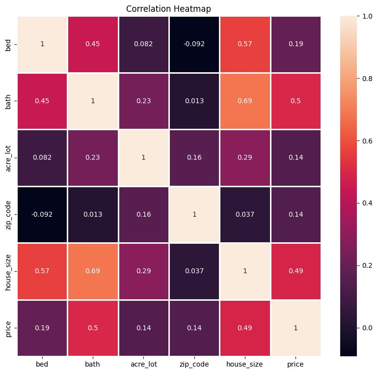
2. We will also plot correlation matrix using heatmap() function to evaluate the relationship between variables. We use the corr() function to determine correlation coefficient between data variables. The value of the correlation coefficient ranges between -1 and +1. The greater the coefficient value, the higher the relationship between variables. A correlation coefficient of 0 indicates no significant linear relationship between variables. The minus value of correlation coefficient indicates that one variable corresponds to a proportional decrease in the other variable, and vice versa with the positive value of the correlation coefficient. The correlation between two same variables will be high because they have same data points. Bath and house_prize have higher correlation than other features with the target.
   
   
   Because bed, acre_lot, and zip_code have low correlation with the target (price), so we need to drop these variables from DataFrame and remains bath and house_size attributes. This result will be assign to X variable. The target will be assigned to y variable.
   
   Print data from variable X and variable y
    
3. We will detect the possibility of multicollinearity with VIF. Multicollinearity refers to a high correlation or linear relationship between two or more independent variables (predictor variables) in a regression model. It occurs when there is a strong association or redundancy among the predictor variables, making it challenging to separate their individual effects on the dependent variable. it can cause several issues in our regression analysis. It turns out that bath and house_size have very high values of VIF, indicating that these two variables are highly correlated, so we need to drop one of these variables from variable X.
   
   We remain house_size data to used in creating the learning model.
   

MODELING

We will create Linear Regression Model.

1. Split the dataset randomly into training and testing subsets. Training data is used to train the model and testing data is used to predict the response and evaluate the model. We will use train_test_split function from sklearn library to perform this splitting. We use 20% of data for testing and remaining 80% for training. We save this splitting as training data (X_train), testing data (X_test), training label (y_train), and testing label (y_test).
   
2. We will create linear regression model using sklearn library. Numpy library is used to convert a variable into an array. To start training the model, we use .fit() function. Because we only have single feature, we need to reshape our data into a 2-dimensional array with a single column using array.reshape(-1,1).
   
3. Make prediction using our trained regression model. We will obtain the predicted response for the test data. The function of .reshape(-1,1) is to ensure that the test data is in the 2-dimensional array format with a single column. Then, we print the predicted values.
   
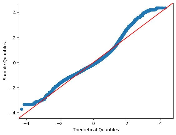
4. We can plot our model using residual and QQ-plot as shown below. For this plotting, we need to import statsmodels library into our workspace.
   
   
   
   

EVALUATION

Every created model need to be proved the validity and reliability of the model using several performance evaluation technique. For evaluating regression model, we can use Mean Squared Error (MSE), Mean Absolute Percentage Error (MAPE), R-Squared Error, and Means Absolute Error (MAE). A lower MSE, MAPE, MAE indicates a better fit of the regression model to the data. On the contrary, higher R² values indicates a good model.

• The MSE score of 75537060315.23729 indicates that there is a significant amount of error between the predicted and actual values, suggesting that the model's predictive accuracy may not be optimal.
• The R-squared score of 0.24023963406173876 indicates that the model explains only a small portion of the variance in the dependent variable, indicating that it may not capture the underlying relationships well.

In conclusion, it is better to perform some improvements in the model's performance, for example using other alternative models, adding independent variables, or refining the existing model to achieve better predictions.