Description

Description

1. Import library

      Here I will import the libraries that I will be using in my notebook. Libraries are essentially extensions to Python that consist of functions         that are handy to have when we are performing our analysis.

2. Import and read data

      Now import and read the 3 datasets as outlined in the introduction.

Note that the test set has one column less than training set, the Survived column. This is because Survived is our response variable, or sometimes called a target variable. Our job is to analyse the data in the training set and predict the survival of the passengers in the test set.

So, our final dataframe that is to be submitted should look something like this, 418 rows and 2 columns, one for PassengerId and one for Survived.

3. Data description

Here I will outline the definitions of the columns in the titanic dataset. You can find this information under the data tab of the competition page.

1. Survived: 0 = Did not survive, 1 = Survived
2. Pclass: Ticket class where 1 = First class, 2 = Second class, 3 = Third class. This can also be seen as a proxy for socio-economic status.
3. Sex: Male or female
4. Age: Age in years, fractional if less than 1
5. SibSp: Number of siblings or spouses aboard the titanic
6. Parch: Number of parents or children aboard the titanic
7. Ticket: Passenger ticket number
8. Fare: Passenger fare
9. Cabin: Cabin number
10. Embarked: Point of embarkation where C = Cherbourg, Q = Queenstown, S = Southampton

4. Exploratory Data Analysis (EDA)

Exploratory data analysis is the process of visualising and analysing data to extract insights. In other words, we want to summarise important characteristics and trends in our data in order to gain a better understanding of our dataset.

   a. Data types, missing data and summary statistics

Seems like Age, Cabin and Embarked colummns in the training set have missing data while Age, Fare and Cabin in the test set have missing data. Another way to to diagnose this is via the missingno library.

   b. Feature analysis

A dataframe is made up of rows and columns. Number of rows correspond to the number of observations in our dataset whereas columns, sometimes called features, represent characteristics that help describe these observations. In our dataset, rows are the passengers on the titanic whereas columns are the features that describe the passengers like their age, gender etc.

Before we move on, it is also important to note the difference between a categorical variable and a numerical variable. Categorical variables, as the name suggests, have values belonging to one of two or more categories and there is usually no intrinsic ordering to these categories. An example of this in our data is the Sex feature. Every passenger is distinctly classified as either male or female. Numerical variables, on the other hand, have a continuous distribution. Some examples of numerical variables are the Age and Fare features.

Knowing if a feature is a numerical variable or categorical variable helps us structure our analysis more properly. For instance, it doesn't make sense to calculate the average of a categorical variable such as gender simply because gender is a binary classification and therefore has no intrinsic ordering to its values.

In this next section of the notebook, we will analyse the features in our dataset individually and see how they correlate with survival probability.

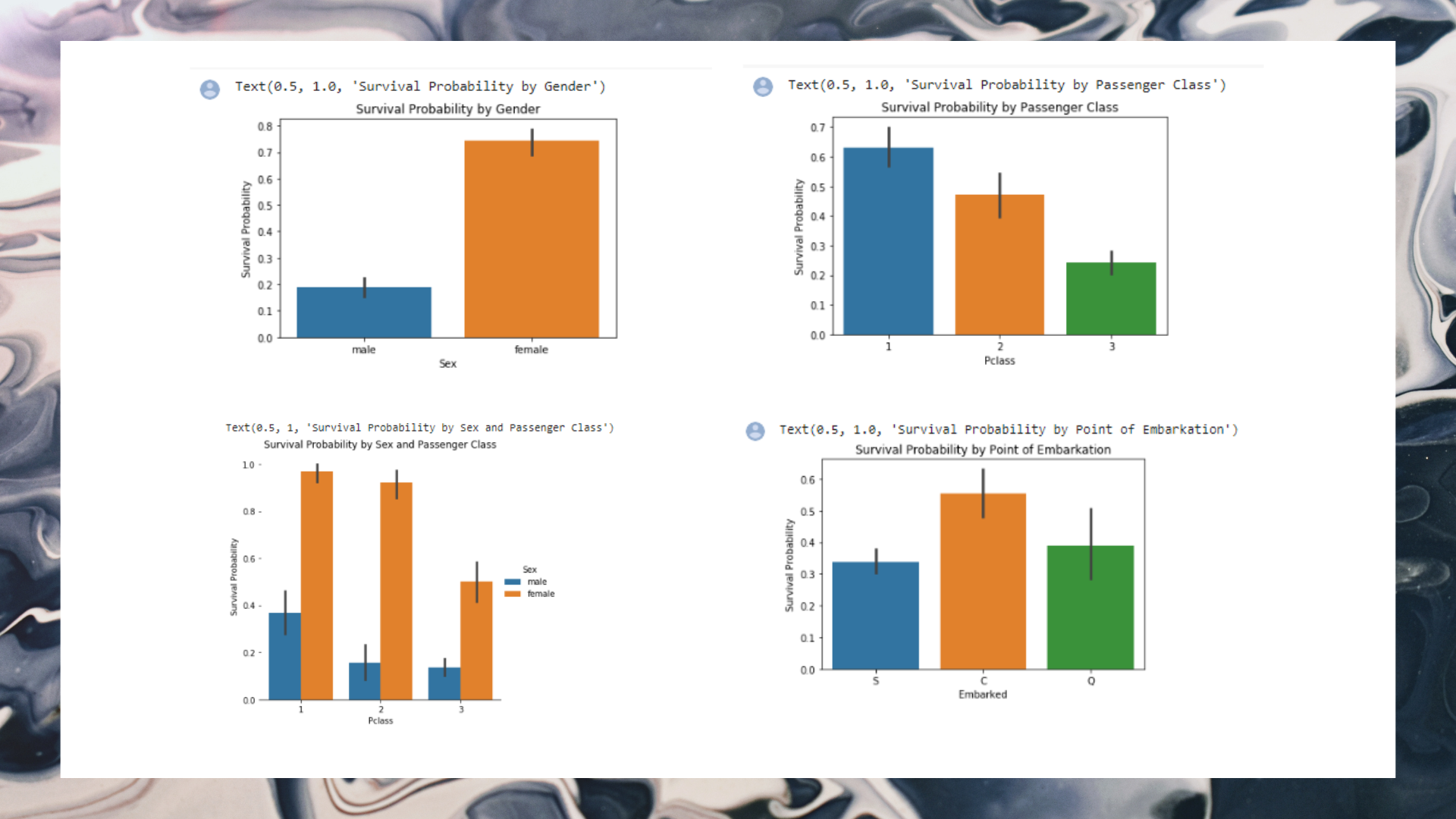
   c. Categorical variables

          1) Categorial variable: Sex

     Categorical variables in our dataset are Sex, Pclass and Embarked.

          2) Categorical variable: Pclass

          3) Categorical variable: Embarked

Survival probability is highest for location C and lowest for location S. Is there a reason for this occurence? We can formulate a hypothesis whereby the majority of the first class passengers have embarked from location C and because they have a highest survival probability, this has resulted in location C having a highest survival probability. Alternatively, there could have been more third class passengers that embarked from location S and because they have the lowest survival probability, this has caused location S to have the lowest survival probability. Let us now test this hypothesis.

Our hypothesis appears to be true. Location S has the most third class passengers whereas location C has the most first class passengers.

5. Data preprocessing

       Data preprocessing is the process of getting our dataset ready for model training. In this section, we will perform the following                        preprocessing steps:

     a. Drop and fill missing values

    I have decided to drop both ticket and cabin for simplicity of this tutorial but if you have the time, I would recommend going through     them and see if they can help improve your model.

       We can ignore missing values in the Survived column because all of them are from the test set. Now we need to fill missing values         in the Age column. The goal is to use features that are most correlated with Age to predict the values for Age. But first, we need to         convert Sex into numerical values where 0 = male and 1 = female. This process is known as encoding and we will further explore this       later in the notebook.

       Age is not correlated with Sex but is negatively correlated with SibSp, Parch and Pclass.

      Loop through each missing age in the list to locate the rows that have the same SibSp, Parch and PClass values and fill the missing           age with the median of those rows. If rows are not found, simply fill the missing age with the median of the entire Age column.

    b. Data trasformation (log transformation)

    Recall that our passenger fare column has a very high positive skewness. Therefore, we will apply a log transformation to address this     issue.

6. Modelling

 Scikit-learn is one of the most popular libraries for machine learning in Python and that is what we will use in the modelling part of this  project. Since Titanic is a classfication problem, we will need to use classfication models, also known as classifiers, to train on our model  to make predictions. I highly recommend checking out this scikit-learn documentation for more information on the different machine  learning models available in their library. I have chosen the following classifiers for the job:

    a. Split training data

    b. Fit model to data and make predictions

This requires 3 simple steps: instantiate the model, fit the model to the training set and predict the data in test set. In this section of the notebook, I will fit the models to the training set as outlined above and evaluate their accuracy at making predictions. Once the best model is determined, I will also do hyperparameter tuning to further boost the performance of the best model.

             1) Logistic regression

             2) Support vector machines

             3) K-nearest neighbours

            4) Gaussian naive bayes

             5) Decisson tree

            6) Random forest

7. Data preprocessing

  Once all our models have been trained, the next step is to assess the performance of these models and select the one which has the           highest prediction accuracy.

 a. Training accuracy

Training accuracy shows how well our model has learned from the training set.

     b. K-fold cross validation

It is important to not get too carried away with models with impressive training accuracy as what we should focus on instead is the model's ability to predict out-of-samples data, in other words, data our model has not seen before.

This is where k-fold cross validation comes in. K-fold cross validation is a technique whereby a subset of our training set is kept aside and will act as holdout set for testing purposes. Here is a great video explaining the concept in more detail.

8. Conclusion

You should achieve a submission score of 0.77511 if you follow exactly what I have done in this notebook. In other words, I have correctly predicted 77.5% of the test set. I highly encourage you to work through this project again and see if you can improve on this result.

Link Datasets : https://www.kaggle.com/c/titanic 

Link Google Colab: https://colab.research.google.com/drive/1sMfa5y1wsziMs1P5B8q6SmTnjFxmsky?usp=sharing