Description

A Python library is a collection of related modules. It contains bundles of code that can be used repeatedly in different programs. It makes Python Programming simpler and convenient for the programmer. As we don't need to write the same code again and again for different programs.

In this notebook, we will be using the following libraries.

In this section, I will fetch the dataset that is available in my Google Drive folder.

The dataset obtained on this link https://www.kaggle.com/datasets/gagandeep16/car-sales

The training set should be used to build your machine learning models. For the training set, we provide the outcome (also known as the “ground truth”) for each Car model. Your model will be based on “features” like Manufacturer, Model, Vehicle Type, Horsepower etc. You can also use feature engineering to create new features.

The test set should be used to see how well your model performs on unseen data. For the test set, we do not provide the ground truth. It is your job to predict these outcomes. For each car, our task is to predict the sales price of the car.

Exploratory Data Analysis refers to the critical process of performing initial investigations on data so as to discover patterns,to spot anomalies,to test hypothesis and to check assumptions with the help of summary statistics and graphical representations.

Here, we will perform EDA on the categorical columns of the dataset - Manufacturer, Vehicle_type and the numerical columns of the dataset - Sales_in_thousands, __year_resale_value, Price_in_thousands, Engine_size, Horsepower, Wheelbase, Width, Length, Curb_weight, Fuel_capacity, Fuel_efficiency, Power_perf_factor.

Here, the columns - Manufacturer, Model, Vehicle_type are categorical. Hence, we modify the datatype of these columns to category.

Looking at the modified datatypes of the columns in the dataset.

From the above data it is evident that there are missing values in the dataset.

From the above dataset, we can see that there are missing values in the column - __year_resale_value, Price_in_thousands, Engine_size, Horsepower, Wheelbase, Width, Length, Curb_weight, Fuel_capacity, Fuel_efficiency, Power_perf_facto

From the above graph, we can see that the number of occurences of the car manufacturers is not uniformly distributed.

From the above graph, we can see that most of the values in the column are Passenger.

From the above graph, we can see that the mean sales price is similar for both the vehicle types.

From the above graph, we can see that the data is slightly skewed. We will remove this skewness during the Data Preprocessing phase.

From the above graph, we can see that the data is slightly skewed. We will remove this skewness during the Data Preprocessing phase.

From the above graph, we can see that the data is slightly skewed. We will remove this skewness during the Data Preprocessing phase.

From the above graph, we can see that the data is slightly skewed. We will remove this skewness during the Data Preprocessing phase.

From the above graph, we can see that the data is slightly skewed. We will remove this skewness during the Data Preprocessing phase.

From the above graph, we can see that the data is normally distributed.

From the above graph, we can see that the data is normally distributed.

From the above graph, we can see that the data is normally distributed.

From the above graph, we can see that the data is slightly skewed. We will remove this skewness during the Data Preprocessing phase.

From the above graph, we can see that the data is normally distributed.

From the above graph, we can see that the data is slightly skewed. We will remove this skewness during the Data Preprocessing phase.

Data preprocessing is the process of getting our dataset ready for model training. In this section, we will perform the following preprocessing steps:

1. Detect and remove outliers in numerical variables
2. Drop and fill missing values
3. Feature Engineering
4. Data Trasformation
5. Feature Encoding
6. Feature Selection

Outliers are data points that have extreme values and they do not conform with the majority of the data. It is important to address this because outliers tend to skew our data towards extremes and can cause inaccurate model predictions. I will use the Tukey method to remove these outliers.

Here, we will write a function that will loop through a list of features and detect outliers in each one of those features. In each loop, a data point is deemed an outlier if it is less than the first quartile minus the outlier step or exceeds third quartile plus the outlier step. The outlier step is defined as 1.5 times the interquartile range. Once the outliers have been determined for one feature, their indices will be stored in a list before proceeding to the next feature and the process repeats until the very last feature is completed. Finally, using the list with outlier indices, we will count the frequencies of the index numbers and return them if their frequency exceeds n times.

From the above cell, we can see that there are no outliers in the data.

We will first remove the records that have missing Price_in_thousands.

From the modified dataset, we can see that there are missing values in the columns - __year_resale_value, Fuel_efficiency, Curb_weight.

Here, we will drop the columns - Model from the dataset.

Feature engineering is arguably the most important art in machine learning. It is the process of creating new features from existing features to better represent the underlying problem to the predictive models resulting in improved model accuracy on unseen data.

Here, we focus on creating new columns for:

1. NewManufacturer - using the column Manufacturer
2. Age - using the column Latest_Launch

Here, we will create the NewManufacturer column such that if the mean price of a Manufacturer is less than 30 then it belongs to class 1, else class 2.

Here, we will create the Age column using the formula 2022 - year value.

From the above graph, we can see that there are only 3 main values for this column

In this section, we will remove the skewness present in the columns - Sales_in_thousands, __year_resale_value, Engine_size, Horsepower, Fuel_capacity, Power_perf_factor by using a Box-Cox transformation on the data. Then, we will normalize all the numerical columns apart from the Target using MinMax Normalization.

From the above graph, we can see that most of the skewness is removed.

From the above graph, we can see that most of the skewness is removed.

From the above graph, we can see that most of the skewness is removed.

From the above graph, we can see that most of the skewness is removed.

From the above graph, we can see that most of the skewness is removed.

From the above graph, we can see that most of the skewness is removed.

Feature encoding is the process of turning categorical data in a dataset into numerical data. It is essential that we perform feature encoding because most machine learning models can only interpret numerical data and not data in text form.

Here, we will use One Hot Encoding for the columns - Manufacturer, Vehicle_type.

Feature selection is the process of reducing the number of input variables when developing a predictive model. It is desirable to reduce the number of input variables to both reduce the computational cost of modeling and, in some cases, to improve the performance of the model.

From the above correlation matrix, we can see that there are a few strong correlations between the data. We will use VIF to remove the multi collinearity.

From the above data, we can see that the columns - Engine_size, Horsepower, Curb_weight, Fuel_capacity, Power_perf_factor cause multicollinearity.

Scikit-learn is one of the most popular libraries for machine learning in Python and that is what we will use in the modelling part of this project.

Since Car Price Prediction is a regression problem, we will need to use regression models, also known as regressors, to train on our model to make predictions. I highly recommend checking out the scikit-learn documentation for more information on the different machine learning models available in their library. I have chosen the following regression models for the job:

1. Multi Linear Regression
2. Lasso Regression
3. Ridge Regression
4. Support Vector Regression
5. Decision Tree regression
6. Random Forest Regression
7. Stacking Regression
8. XGBoost Regression

In this section of the notebook, I will fit the models to the training set as outlined above and evaluate their Root Mean Squared Error (RMSE), R-squared at making predictions. Then, we will select the best model based on those values.

Here, we will split the training data into X_train, X_test, Y_train, and Y_test so that they can be fed to the machine learning models that are used in the next section. Then the model with the best performance will be used to predict the result on the given test dataset.

Now, we apply regressors using the above data.

Model evaluation is the process of using different evaluation metrics to understand a machine learning model's performance, as well as its strengths and weaknesses.

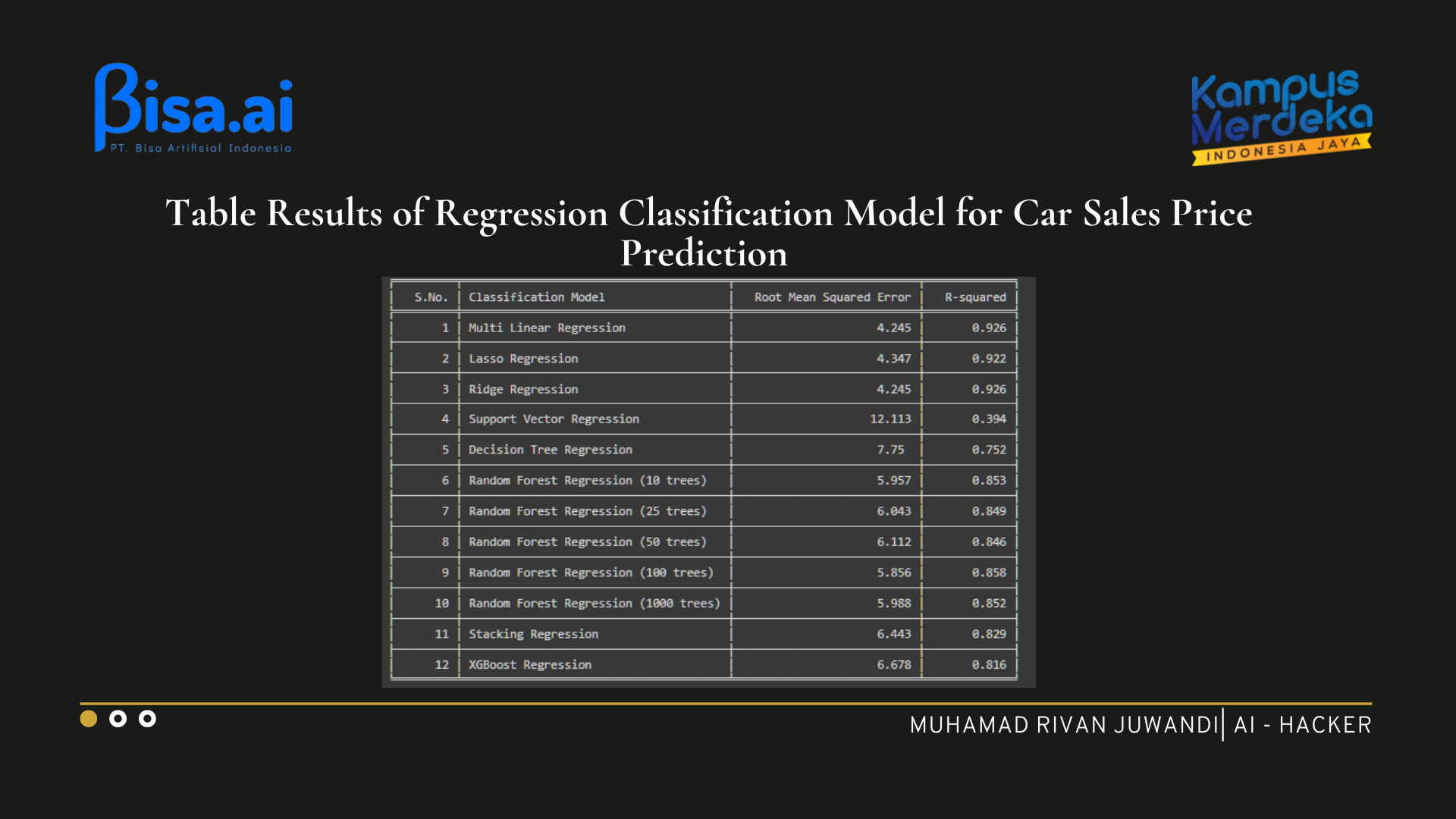
Now we will tabulate all the models along with their RMSE, R-Squared. This data is stored in the model_rmse, model_r2 dictionary. We will use the tabulate package for tabulating the results.

From the above table, we can see that the model Linear Regression has the least Root Mean Squared Error of 4.245 and the highest R-squared value of 0.926.

Hence, for this problem, we will use Linear regressor to predict the Sales Price of the Car.