Comparison of Classification models for Glaucoma
Aditya Paramananda

Summary
Glaucoma attacks people from young to old age. Generally, this disease can attack people who suffer from diabetes and hypertension. And also, hereditary factors can also be the main factor in developing glaucoma. Glaucoma is also a disease that cannot be cured at this time and has many factors. Therefore, researchers can classify glaucoma disease and find the accuracy value in classifying the disease. In classifying diseases, researchers use several variables to search based on the existing diagnosis. To know that this diagnosis can be classified, you need to use machine learning classification methods. Therefore, researchers used Naïve Bayes, Random Forest, and KNN methods to classify glaucoma. The results of this research are that the KNN method obtains the best results compared to others. The Naïve Bayes method obtained 50% and the Random Forest method obtained 50%. KNN obtained accuracy results of 55% with split data of 60% training and 40% testing.
Description
1. Datasets
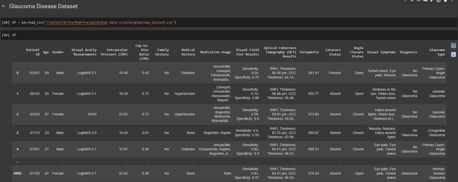
This dataset contains data on patients with glaucoma. This dataset contains 10,000 data records used for glaucoma disease detection. This dataset contains:
A. Patient ID
B. Age
C. Gender
D. Visual Acuity Measurements
E. Intraocular Pressure (IOP)
F. Cup-to-Disc Ratio (CDR)
G. Family History
H. Medical History
I. Medication Usage
J. Visual Field Test Results
K. Optical Coherence Tomography (OCT) Results
L. Pachymetry
M. Cataract Status
N. Angle Closure Status
O. Visual Symptoms
P. Diagnosis
Q. Glaucoma Type
2. Method
A. Dataset
The first step that researchers take is selecting a dataset to study. Researchers chose a dataset from Kaggle which contained glaucoma sufferers. This data contains a total of 10,000 data on patients suffering from glaucoma. The purpose of choosing this dataset is to be able to classify glaucoma disease based on the diagnostic variables in the data. Next, get into coding by starting to create a library.
B. Library for the classification of Glaucoma

The first step before getting to the data is to write the libraries used in the classification of Glaucoma disease. The library contains basic libraries for analysis such as pandas, numpy, seaborn, and matplotlib. Then it is also used for modelling and evaluation processes. The modelling process contains classification models such as Naïve Bayes, KNN, and Random Forest. The evaluation used is using accuracy values as evaluation in this research. The next step is to display the data.
C. Displaying Data

The third step is to display the Glaucoma disease dataset. Previously, researchers took data from Kaggle. Researchers downloaded the data in CSV file format. So by using .csv, researchers use the pandas library, namely read_csv(). Researchers obtained 10,000 data according to the description on Kaggle. Next is to drop the “patient ID” for privacy.
D. Drop Variable “Patient ID”

The fourth step is Remove "patient ID" from the data because "patient ID" is a form of privacy that must be kept confidential and is not really used in this research. By deleting this, the variables currently used are used for data analysis. Next is to display dataset info and dataset description.
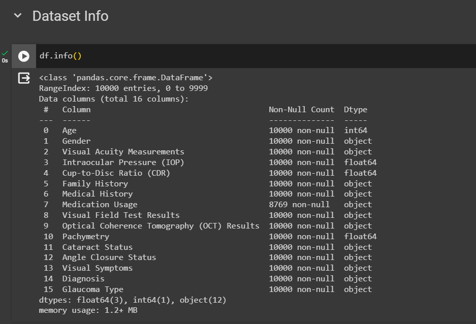
E. Dataset Info and Dataset Description

The next step is to see in the picture above that each variable in the dataset has a different data type. The most common data type in this data is using objects or categories compared to numeric. So, from this information, before entering the model section, researchers need to change the categorical data to numerical data to be able to find correlation and accuracy values.

The data description contains numerical data which can be presented with mean, max, standard deviation, etc. The numerical data in the dataset are the variables Age, IOP, CDR, and Pachymetry. From this numerical data, the relationship with diagnosis will later be analysed. Next is to check for empty values in the dataset.
F. Check Missing Value and Clean Missing Value.

Missing values in this dataset total 1231 in the variable "Medication Usage". Therefore, the researcher made improvements by removing empty parts in the data with the function in Pandas, namely drop.na. By using drop.na, the dataset is free from missing values
G. Analysis Data
At this stage, researchers carried out several analyses that were used to classify glaucoma. Before entering into analysis of the data, Exploratory data analysis (EDA) was carried out at the initial stage such as dropping the Patient ID variable, and checking for missing values in the data. Now we explain the analysis of categorical data and numerical data in the dataset, then explain the correlation between variable relationships by changing categories to numerical. The first is to look at the data distribution in numerical data. Numerical data in this dataset include age, Cup-to-Disc Ratio (CDR), Intraocular Pressure (IOP), and Pachymetry. The following is a visualization of data distribution in numerical data.


Figures above are visualizations of data distribution in numerical data. Next is analysis of categorical data. Data categories in this dataset used for this research include gender, visual acuity measurements, family history, medical history, cataract status, angel closure status, and diagnosis. I chose this category of data because I wanted to see which factors could be used as benchmarks for a diagnosis of glaucoma. The following is a visualization of the category data in this dataset.

In this gender category, the number of males is 4406, and for females it is 4363 in data from patients suffering from glaucoma.

In the Visual Acuity Measurements category there were LogMAR 0.0 is 2235, LogMAR 0.1 is 2196, 20/20 is 2183, and 20/40 is 2155.

In this section, glaucoma is based on family history. In this category it consists of Yes is 4348, and No is 4421.

In this section, glaucoma is based on medical history. This category consists of None is 2218, Hypertension is 2186, Glaucoma in family is 2184, and Diabetes is 2181.

In this section, glaucoma is based on cataract status. This category consists of Absent is 4460 and Present is 4309.

In this section, glaucoma is based on angle closure status. This category consists of Closed is 4438 and Open is 4331.

In this section, glaucoma is based on diagnosis. This category consists of No Glaucoma is 4387, and Glaucoma is 4382. Next is data analysis combined with several categorical variables. Following is the analysis and visualization of category data with diagnosis.

Figure above is a visualization of the influence of gender and age on diagnosis. It can be seen in figure 18 that men have the most glaucoma sufferers compared to women. So, in this dataset, male is more susceptible to this disease than female.


Researchers created figures above to find out who had glaucoma at the age of less than 40 and more than 40 years. It turns out that the results are figure above. There are more glaucoma sufferers in men than in women. From this visualization we can see that glaucoma can attack at any age. In the age variable, the youngest age is 18 years old and the oldest is 90 years old. Even though glaucoma sufferers are mostly older, young people must also be able to maintain their health.

Figure above explains the relationship between medical history and diagnosis. It can be seen that in this medical history there are several diseases suffered by the patient. These diseases are Diabetes, Hypertension, None, and Glaucoma in the family. The results in figure above show that there are more people who do not have a medical history than those who have heredity and disease. This indicates that we must maintain health even if we are not affected by disease or are hereditary to prevent glaucoma.

Figure above explains the relationship between visual acuity measurements and diagnosis. As seen in figure above, there are LogMar 0.1, 20/40, LogMar 0.0, and 20/20. The result from figure 22 is that LogMar 0.0 has more glaucoma sufferers than others. LogMar is used to measure a person's visual acuity. LogMar 0.0 means that visual acuity is still mostly normal. However, there is also vision that begins to decrease at LogMar0.1 and 20/40.

Figure above explains the relationship between cataract status and diagnosis. Seen in cataract sufferers can be associated with a diagnosis of Glaucoma. The results of figure above show that there are more Glaucoma sufferers who do not have cataracts than those who have cataracts. So, it can be concluded that when people suffer from glaucoma, most people do not have cataracts and are healthy.

Figure above shows how to change categorical data to numerical data. I replaced it with the numbers 0 and 1 which correspond to the contents of the data. For example, in gender I changed male and female to numbers 0 and 1.


From figure above a heatmap will be created with a correlation function for all data. Figure above is a heatmap of the data that was determined at the beginning. From this data, we want to see the relationship between diagnosis and all variables. It appears that the diagnosis is closely correlated with cataract status. And the diagnosis is too far from age. However, this data is too far from the diagnosis.
H. Split Data
Researchers split the data from 90% training and 10% testing to 60% training and 40% testing. Split data is carried out to evaluate whether the model created can produce high accuracy values or not. The results are displayed in the results section

I. Model
This stage is a continuation of split data. After splitting the data, the researchers initiated the Naïve Bayes, Random Forest, and KNN models. The model will be initialized according to the provided python library.


J. Evaluation
To assess whether the model is good or not through evaluation. After the model process is complete, the next step is evaluation. This research uses evaluation based on accuracy values. Each model looks for evaluation values from each split data. The exact results will differ according to the data split that has been initiated. The results of the evaluation are explained in the results section.
3. Result
No | Model | Split Data | Accuracy |
1 | Naïve Bayes | 90 Training, 10 Testing | 0.5371 |
|
| 80 Training, 20 Testing | 0.5120 |
|
| 70 Training, 30 Testing | 0.5101 |
|
| 60 Training, 40 Testing | 0.5034 |
2 | Random Forest | 90 Training, 10 Testing | 0.5143 |
|
| 80 Training, 20 Testing | 0.5108 |
|
| 70 Training, 30 Testing | 0.4907 |
|
| 60 Training, 40 Testing | 0.5008 |
3 | KNN | 90 Training, 10 Testing | 0.5416 |
|
| 80 Training, 20 Testing | 0.5381 |
|
| 70 Training, 30 Testing | 0.5484 |
|
| 60 Training, 40 Testing | 0.5524 |
Table Above is the model results evaluated using accuracy. This accuracy is obtained from various data splits. The split data used in this research included 90% training 10% testing, 80% training and 20% testing, 70% training 30% testing, and 60% training 40% testing. The worst result in model comparison lies in the random forest model with a result of 0.4907 with a data split of 70% training and 30% testing. The best results in model comparison were the use of classification in KNN with a result of 0.5524 with a data split of 60% training and 40% testing. So, it can be concluded that the best accuracy value is the KNN model with split data of 60% training and 40% testing.
4. Conclusion
The conclusion of this research begins with an analysis of gender, age, and diagnosis. It was found that men were the most sufferers from the Glaucoma dataset. There were 2217 men suffering from glaucoma. Then the sufferers are not only elderly people but also many young people aged 18 years who are already suffering from glaucoma. Then, not only based on age, it turns out that many glaucoma sufferers also have no history of the disease, no cataracts, and normal vision. So, researchers can conclude that even healthy people can also get glaucoma. However, the main factor in developing glaucoma is also not far from diseases such as diabetes, hypertension or family heredity. Then the results of the model evaluation in this research with the best accuracy value were obtained by the KNN model with a value of 55% with split data of 60% training and 40% testing.
Informasi Course Terkait
Kategori: Data Science / Big DataCourse: Persiapan Ujian Sertifikasi Internasional DSBIZ dan AIBIZ