Description

This project discusses the classification of diabetes data with machine learning models. 

What is Diabetes?

Diabetes is a chronic disease that occurs when the pancreas can no longer make insulin or the body cannot make good use of the insulin it produces. Learning how to use Machine Learning can help us predict Diabetes.

About this Project :

• The objective of this project is to classify whether someone has diabetes or not.
• Dataset consists of several Medical Variables(Independent) and one Outcome Variable(Dependent)
• The outcome variable value is either 1 or 0 indicating whether a person has diabetes(1) or not(0).

About the Dataset

• Pregnancies : Number of times a woman has been pregnant
• Glucose : Plasma Glucose concentration of 2 hours in an oral glucose tolerance test
• BloodPressure : Diastolic Blood Pressure (mm hg)
• SkinThickness : Triceps skin fold thickness(mm)
• Insulin : 2-hour serum insulin(mu U/ml)
• BMI : Body Mass Index ((weight in kg/height in m)^2)
• Age : Age(years)
• DiabetesPedigreeFunction : scores likelihood of diabetes based on family history)
• Outcome :- 0(doesn't have diabetes) or 1 (has diabetes)

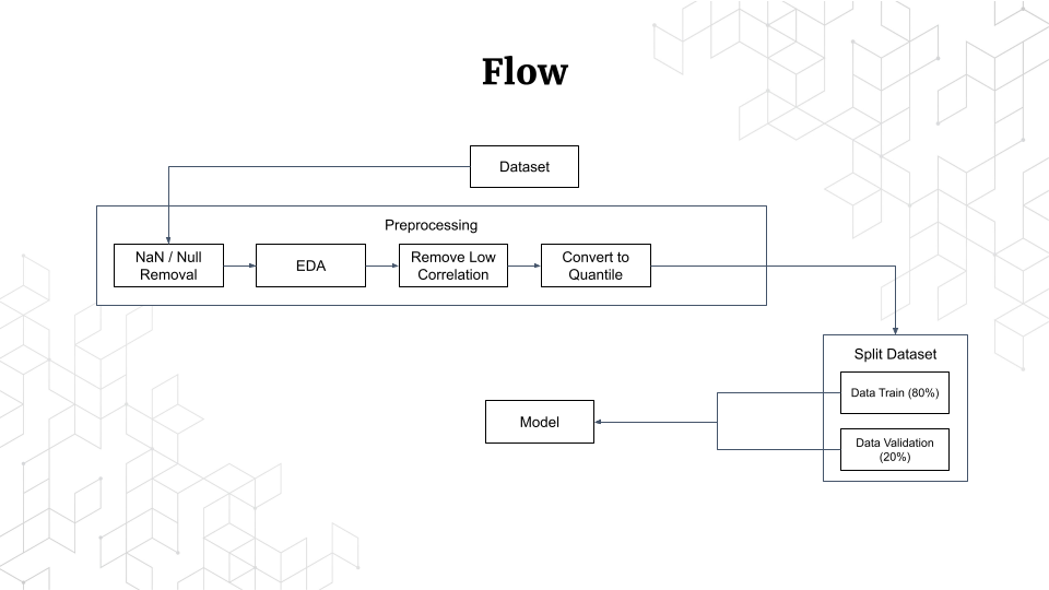
Flow of this Project

we will work based on the flow below, please remember that the flow of each cases of machine learning and the tasks is different, so this flow is not all the machine learning task have a work flow like this.

Preparation

The first thing you can do is download the dataset, you can download this dataset on Kaggle by clicking this link Pima Indians Diabetes Database | Kaggle, after you downloaded it, you can make a folder in your Google Drive and upload it to that folder. After that, you can just make jupyter notebook (ipynb) file in the same folder, if you don't have Google Colaboratory installed yet, you can follow these steps.

Click “+ New”

Click More > Connect more apps

Search for “google colab”

Click install, then you can create the jupyter notebook file

Preprocessing

• Open the ipynb file that you created earlier, then connect the Google Drive to your file by typing this code.

Please remember, since we are using Google Colaboratory, connecting or mounting your Google Drive to your ipynb file is a must thing todo

• Next Import the necessary library

• Load the Dataset

Please remember, location of the dataset file is different, but “/content/drive/My Drive…” section is all the same, the rest you can change to your file location

• Next we see the shape of the dataset

By doing this you can see the shape or you can say the size of the dataset, for example, by the picture below that means this dataset has 768 rows and 9 columns

• Then we remove Duplicated Value and Null Value

You can check whether your dataset has a Null Value or not by typing "df.isnull().sum()" where the code will show the data with a Null Value with isnull() function, and count the total instead of showing the data by sum().

• Next we visualized the dataset

Based on the picture below, we can see that data with diabetes is 268 rows and not diabetes is 500 rows

for the picture below we visualized each column with the value

• For better performance, next we will delete the columns with low correlation with Outcome

as you can see the lowest correlation with Outcome is the Blood Pressure column, Skin Thickness column, and Insulin column, so we remove those columns by typing this code.

• Next we transform all the selected independent values into Quantile Value, which means all the values will be changed into probability

Splitting Dataset

• First we separate the selected data into X and Y variables, where X is the independent columns, and Y is the dependent column

• Then we split the data into train data and test data, with ratio 8:2, and we also see the shape of it just to make sure we have the correct ratio

Implement the Models

• First we will use SVM Model

in this model, we will not only be implementing but also tuning hyper-parameters, by doing this allow the model to perform the most optimal performance, tuning hyper-parameters by typing this code below.

after that, we just fit or implement the model into the data by typing this code below

this will take a bit of time, after the process is completed, it should show a green check mark like that. When this process completed that means our model is trained, all we have to do is do the test and see the score, to test the model, you can type this code

and then we can see the score based on the test that we do just now

as you can see in the f1-score column, we have a 78% accuracy

and the picture above is the confusion matrix, you can read it by seeing the row and column, for example, row 0 means data with 0 values, and column 0 means the predicted data, so the trained model predicted that 83 data with 0 value is labeled with 0 or not diabetes, which means the model predicted right 83 rows, and you can see row 1 and column 0, that means the trained model predicted 18 rows is labeled 0 or not diabetes where the actual label is 1 or positive diabetes, and so on.

• Second we will use Naive Bayes Model

For the Naive Bayes Model, we will also do tuning hyper-parameters and the process also not too different with the previous model

then we fit and test the model

after the process completed we see the score based on the test

as you can see this time with Naive Bayes Model we get 72% Accuracy with confusion matrix like the picture below

• and then the last one we will use Decision Tree Model

For this model we also do tuning hyper-parameters

after the hyper-parameters have been tuned we can fit the model and test it

and then we can see the score and the confusion matrix

as you can see, for this model we get 72% Accuracy with the confusion matrix like the picture below